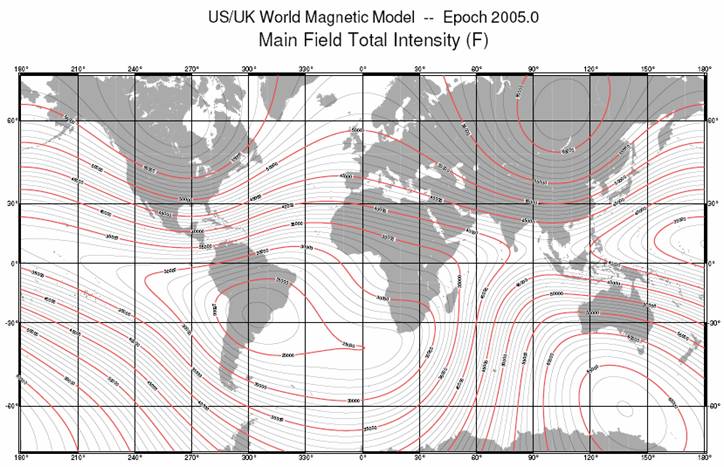
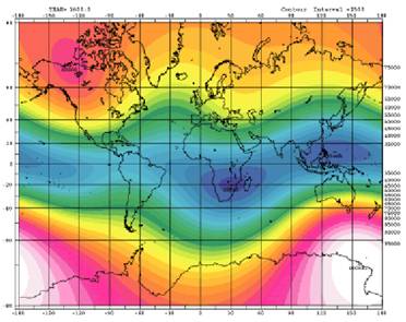
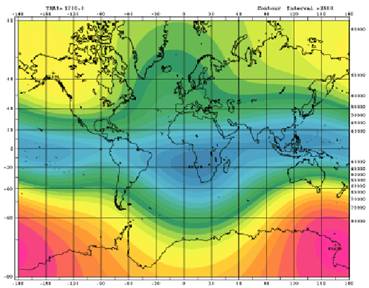
The strength of the Earth’s magnetic field varies tremendously around the world. The following figure shows the magnetic field intensity around the world in 2005 [http://www.ngdc.noaa.gov/geomag/WMM/data/wmm-F05.pdf]. The magnetic field has greatest strength near the poles and the weakest area over South America and across the El Nino area of the Pacific Ocean.

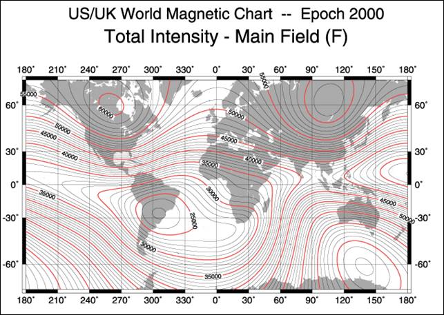
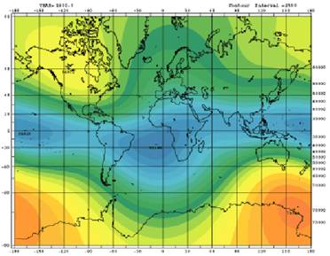
The following figure shows the same as above for the year 2000 [http://www.ngdc.noaa.gov/geomag/icons/wmm2000f.gif]

In the five years from 2000 to 2005 the magnetic field has noticeably changed in a couple of areas:

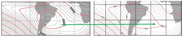
The South Atlantic weak zone has expanded to the east.

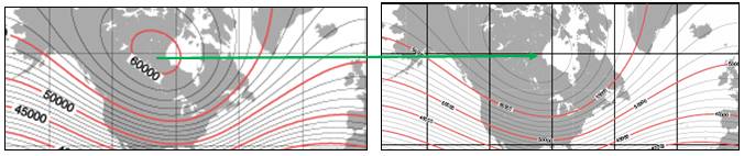
The Northern Canada strong zone has weakened as the north magnetic pole transits to Siberia.

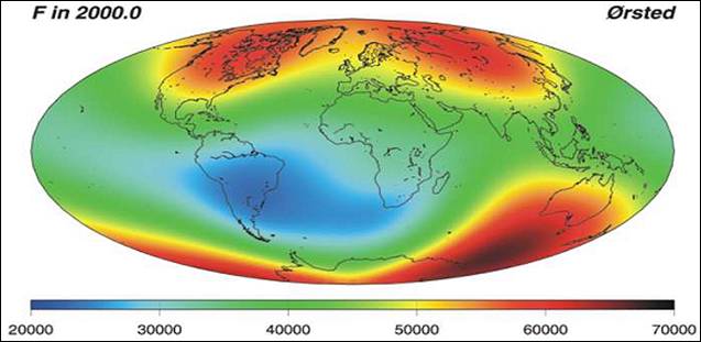
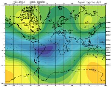
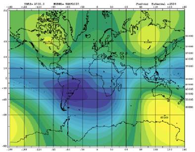
The following figure shows another view of the Earth’s magnetic field intensity in 2000 from the Danish Orsted satellite [http://smsc.cnes.fr/OVH/]

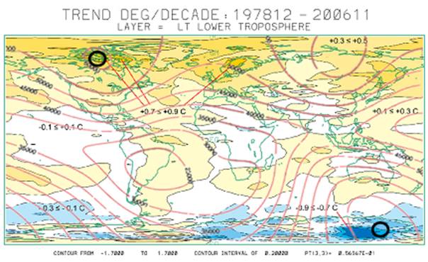
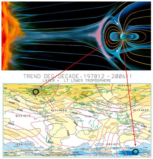
The following figure shows the global temperature change from 1978 to 2006 for the lower troposphere from satellite data [http://climate.uah.edu/25yearbig.jpg]. The red contour lines are the year 2000 magnetic field intensity contours (5000 nT contours) shown previously. The areas of greatest warming are where the magnetic field is at its greatest intensity in the northern polar region, whereas the area of greatest cooling is where the magnetic field is at its greatest intensity in the southern polar region.

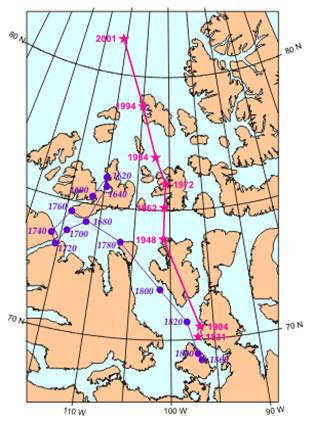
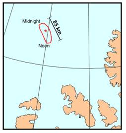
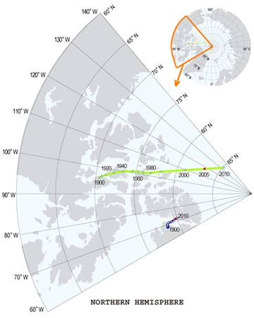
The locations of the magnetic poles are not static and continuously change position. The following figure (left) shows (magenta) the path of the North Magnetic Pole (NMP) since its discovery in 1831 to the last observed position in 2001, and (purple) past NMP positions since approximately 1600 derived from spherical harmonic models. [http://gsc.nrcan.gc.ca/geomag/nmp/long_mvt_nmp_e.php] The figure below right illustrates that the position of the NMP given for a particular year is an average position – it wanders daily around this average position and, on days when the magnetic field is disturbed, may be displaced by 80 km or more. Although the daily motion on any given day is irregular, the average path forms a well-defined oval due to interaction with the sun’s magnetic field.

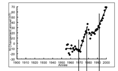
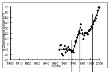
Since about 1970 the NMP has accelerated and is now moving at more than 40 km per year. The following figure shows the average change in motion of the North Magnetic Pole since the 1950s. Since the early 1970s the rate of change of the location increased from about 9 km/yr to 41 km/yr.

A 2005 Oregon State University article “Movement of Earth's North Magnetic Pole Accelerating Rapidly” [http://oregonstate.edu/dept/ncs/newsarch/2005/Dec05/magneticnorth.htm] states: “After some 400 years of relative stability, Earth's North Magnetic Pole has moved nearly 1,100 kilometers out into the Arctic Ocean during the last century and at its present rate could move from northern Canada to Siberia within the next half-century. … the North Magnetic Pole has moved all over the place over the last few thousand years. In general, it moves back and forth between northern Canada and Siberia.”

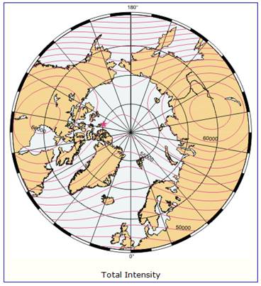
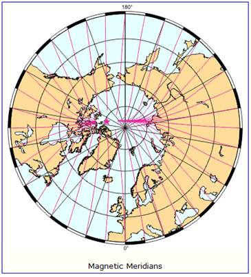
The following figures show the magnetic field intensity (left) and the magnetic meridians (right) [http://gsc.nrcan.gc.ca/geomag/field/arctics_e.php]. The NMP position is indicated by the star. The magnetic field is asymmetrical – with two field maxima: one over the northwest shore of Hudson Bay in Canada, and one over the Central Siberian Plateau. The convergences of the magnetic meridians indicate the approximate path followed by the moving NMP.

The magnetic pole in Northern Canada has been weakening as it shifts across the Arctic to Siberia (total field intensity 2000 (left) and 2005 (right).

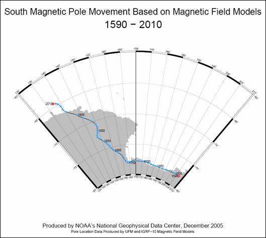
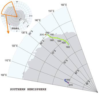
The following figure shows the historical movement of the South Magnetic Pole. [http://www.ngdc.noaa.gov/geomag/maps/SouthPole1590_2010.pdf]

The following figures show movement of the magnetic poles projected to 2010 calculated using the International Geomagnetic Reference Field (IGRF) model [http://swdcwww.kugi.kyoto-u.ac.jp/poles/polesexp.html] The south magnetic pole has not accelerated over the last few decades like the NMP has.

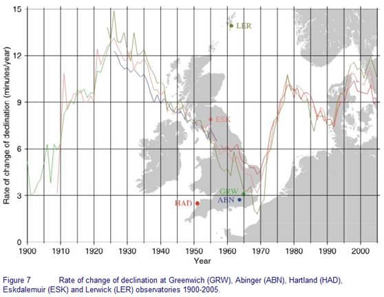
The following figure shows the rate of change of NMP declination at Lerwick, Eskdalemuir and Greenwich-Abinger-Hartland observatories in the United Kingdom. “It can be seen from this plot that there have been a number of changes in the general trend of secular variation in the past, in particular at about 1925, 1969, 1978 and 1992. These sudden changes are known as jerks or impulses and, at the present time, are not well understood and are certainly not predictable. Some researchers have found evidence for a correlation with length-of-day changes.” [http://www.geomag.bgs.ac.uk/earthmag.html]

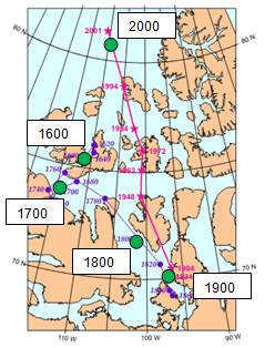
The following sequence of figures shows the change of the magnetic field intensity over the last 400 years derived from IGRF [http://swdcwww.kugi.kyoto-u.ac.jp/igrf/anime/index.html], along with the NMP movement map shown previously. The overall intensity of the magnetic field has decreased. In 1600 there was a more distinct intensity over northern Canada. Over the centuries this has weakened, while increasing over the last century in northern Siberia. As the field intensity increases in Siberia and decreases in Canada, the north magnetic pole moves across the arctic from Canada towards Siberia.

1600                                                                                        1700

1800                                                                                        1900

2000

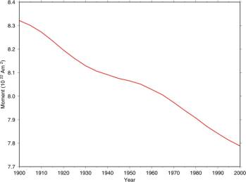
The following figure is from the British Geological Survey [http://www.geomag.bgs.ac.uk/reversals.html], “Measurements have been made of the Earth's magnetic field more or less continuously since about 1840. If we look at the trend in the strength of the magnetic field over this time (for example the so-called 'dipole moment' shown in the graph below) we can see a downward trend. ... We also know from studies of the magnetisation of minerals in ancient clay pots that the Earth's magnetic field was approximately twice as strong in Roman times as it is now.”

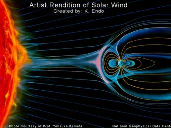
The Earth’s magnetic field “acts as a shield against the bombardment of particles continuously streaming from the sun. Because the solar particles (ions and electrons) are electrically charged, they feel magnetic forces and most are deflected by our planet's magnetic field. However, our magnetic field is a leaky shield and the number of particles breaching this shield depends on the orientation of the sun’s magnetic field. … Twenty times more solar particles cross the Earth’s leaky magnetic shield when the sun’s magnetic field is aligned with that of the Earth compared to when the two magnetic fields are oppositely directed” [http://www.nasa.gov/mission_pages/themis/news/themis_leaky_shield.html]

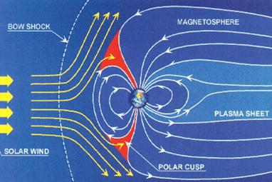
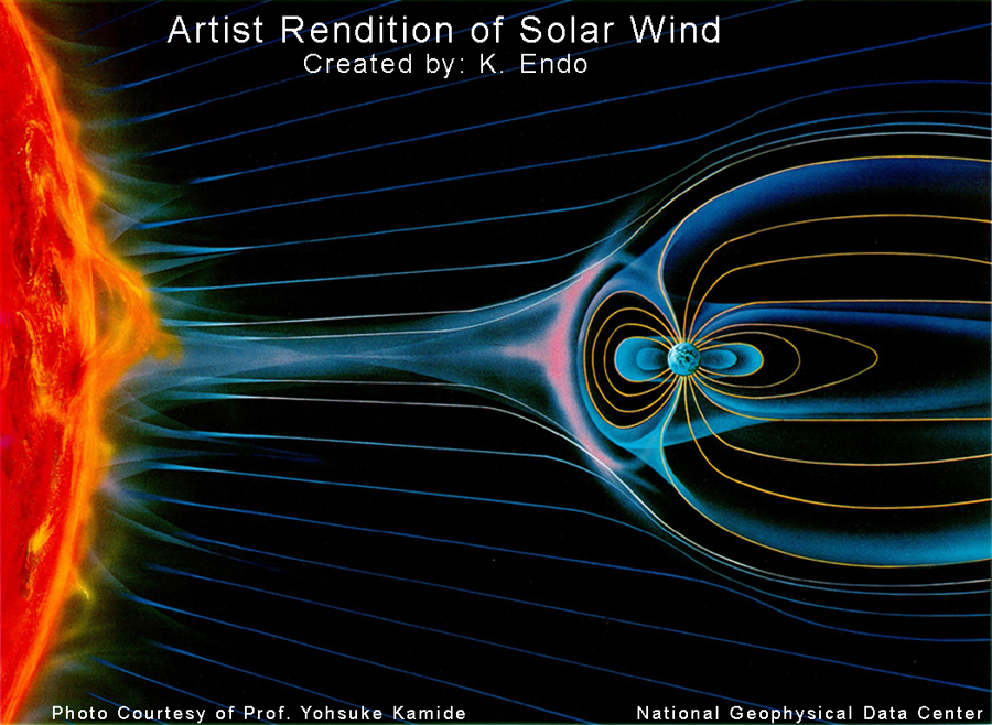
The Earth’s magnetic field interacts with the Sun’s magnetic field. The interplanetary magnetic field (IMF) is a part of the Sun's magnetic field that is carried into interplanetary space by the solar wind. [http://pluto.space.swri.edu/image/glossary/cme.html]. The Earth’s magnetic field is distorted by the solar wind as illustrated by the following figures [http://www.ngdc.noaa.gov/geomag/icons/solarexp.jpg] (left) and [http://smsc.cnes.fr/OVH/] (right)

“Most of the energy transfer to the Earth from the solar wind is accomplished electrically, and nearly the entire voltage associated with this process appears in the polar cap region, which extends typically less than 20° in latitude from the magnetic pole. The total voltage across the polar cap can be as large as 100,000 volts, rivaling that of thunderstorm electrification of the planet in magnitude. This polar cap electric field is the major source of largescale horizontal voltage differences in the atmosphere. Moreover, the dynamic polar region accounts for a large fraction of the variability inherent in our upper atmosphere, variability due to chaotic changes in the solar wind magnetic field that produces large-scale restructuring of the cavity enclosing the Earth’s magnetic field. This restructuring visibly manifests itself most clearly in the production of ionized plasmas and the associated distribution of aurora high over the north and south polar regions. In turn, the Earth’s lower atmosphere (that part responsible for weather phenomena) undergoes variations in composition and dynamics influenced by these coupling effects through a complex and as yet not fully understood feedback system. [http://www.arcus.org/logistics/svalbard/Svalbard.pdf]

“Coronal mass ejections (CMEs) are eruptions into interplanetary space of as much as a few billion tons of plasma and embedded magnetic fields from the Sun's corona. ... The exact processes involved in the release of CMEs are not known. CMEs can occur at any time during the solar cycle, but their occurrence rate increases with increasing solar activity and peaks around solar maximum. ... Fast CMEs --those traveling faster than the ambient solar wind-- are responsible for triggering large, nonrecurrent geomagnetic storms when they encounter the Earth's magnetosphere. Such storms can result from the passage either of the CME itself or of the shock created by the fast CME's interaction with the slower-moving solar wind. The majority of large and major geomagnetic storms are generated by the encounter with both the interplanetary shock and the CME that drives it. The "geoeffectiveness" of CMEs --i.e., their ability to disturb the Earth's magnetosphere-- is a function of their speed, the strength of their magnetic field, and the presence of a strong southward magnetic field component.” [http://pluto.space.swri.edu/image/glossary/cme.html].

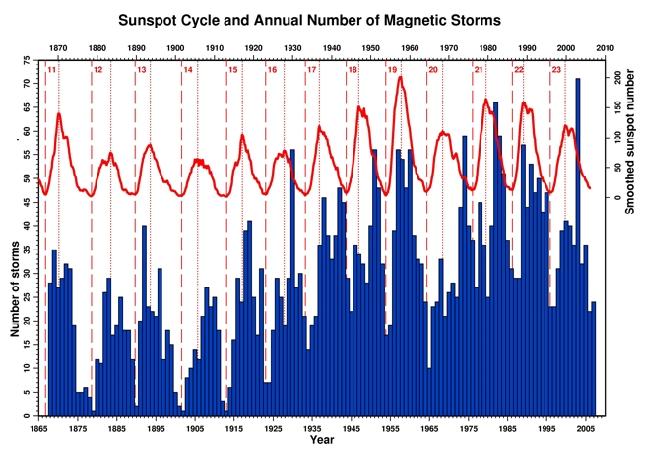
The following figure shows the correspondence of solar geomagnetic storms and the solar sunspot cycle [http://www.geomag.bgs.ac.uk/earthmag.html].

A study done by an Assistant Professor of Earth Sciences at Dartmouth University [http://www.sciencedaily.com/releases/2002/06/020607073439.htm] looked at the cycles of the sun’s magnetic fluctuations and found: “when the sun is magnetically more active, the earth experiences a warmer climate, and vice versa, when the sun is magnetically less active, there is a glacial period. Right now, the earth is in an interglacial period (in between ice ages) that began about 11,000 years ago, and as expected, this is also a time when the estimated solar activity appears to be high”

Authors of a Danish study published in 2009 stated: “Our results show a strong correlation between the strength of the earth's magnetic field and the amount of precipitation in the tropics” [http://www.physorg.com/news151003157.html]

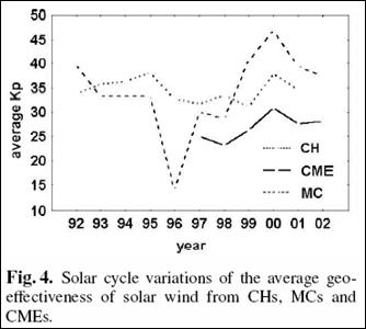
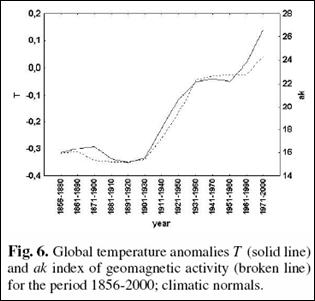
A 2005 study (Georgieva, Bianchi and Kirov: “Once Again About Global Warming and Solar Activity”, Mem. Societa Astronomica Italiana, Vol 76, 2005 [http://sait.oat.ts.astro.it/MSAIt760405/PDF/2005MmSAI..76..969G.pdf]) states: “We show that the index commonly used for quantifying long-term changes in solar activity, the sunspot number, accounts for only one part of solar activity and using this index leads to the underestimation of the role of solar activity in the global warming in the recent decades. A more suitable index is the geomagnetic activity which reflects all solar activity, and it is highly correlated to global temperature variations in the whole period for which we have data.” The study examined the geoeffectiveness of coronal mass ejections (CME) separated into two types – magnetic cloud (MC) and non-MC CMEs (CME), and coronal holes (CH). “when speaking about the influence of solar activity on the Earth, we cannot neglect the contribution of the solar wind originating from coronal holes. However, these open magnetic field regions are not connected in any way to sunspots, so their contribution is totally neglected when we use the sunspot number as a measure of solar activity” The following figures are from their study.

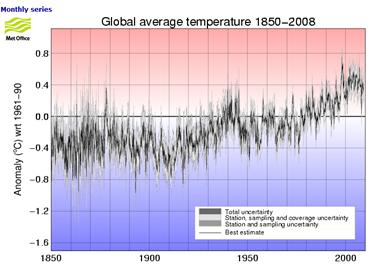
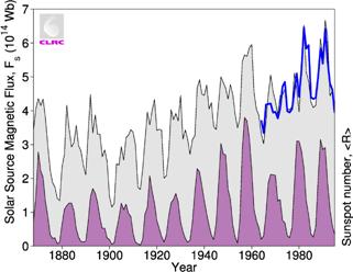
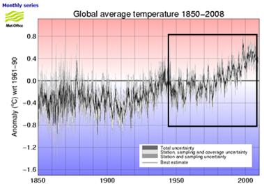
The following figures show the global average temperature from 1850 – 2008 (left) [http://hadobs.metoffice.com/hadcrut3/diagnostics/global/nh+sh/], and (right) the total solar magnetic flux (black line bounding grey shading and blue line) along with the annual sunspot number (shaded purple). The solar figure is from M. Lockwood, R. Stamper, and M.N. Wild: “A Doubling of the Sun's Coronal Magnetic Field during the Last 100 Years”, Nature Vol. 399, 3 June 1999 [http://www.ukssdc.ac.uk/wdcc1/papers/nature.html]) which states: “The magnetic flux in the solar corona has risen by 40% since 1964 and by a factor of 2.3 since 1901.”

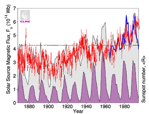
The following figure superimposes the global temperature (from above left – changed to red) on the solar flux (from above right).

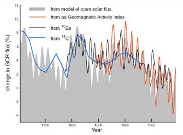
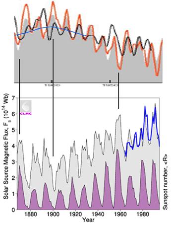
The following figure shows the change in global cosmic ray flux (GCR) from four independent proxies (left) showing the decrease in GCR throughout the 1900s. [http://meteo.lcd.lu/globalwarming/Gray/Influence_of_Solar_Changes_HCTN_62.pdf] The right-hand figure compares the same data with the solar magnetic flux from above, showing the strong inverse correlation between the solar magnetic flux and the cosmic ray flux. The figures above and below indicate a strong correlation between the solar magnetic flux, the cosmic ray flux, and the global temperatures.

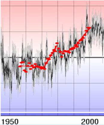
The following figures show global average temperature (left) and the average change in motion of the North Magnetic Pole (right) as shown previously. The next figure below combines these two, with the North Magnetic Pole data changed to red. There is a clear correlation between the rate of change of the North Magnetic Pole location and the global temperature.

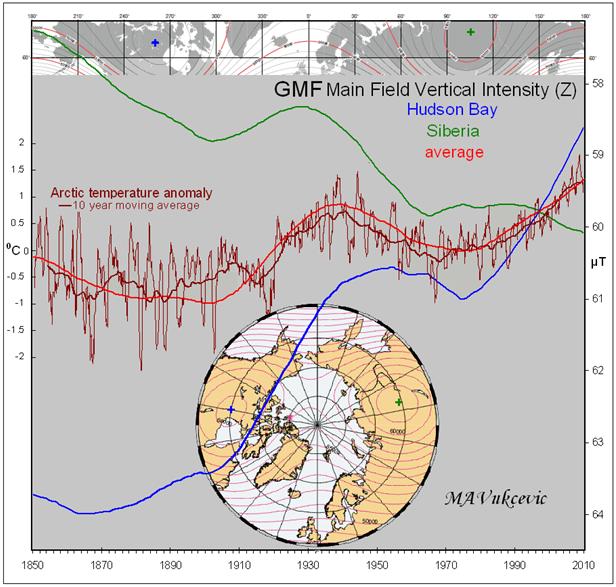
The following figure shows the correspondence between the changing magnetic field in the Arctic and Arctic temperatures. The magnetic field is shown for Hudson Bay (blue), Siberia (green) and the average (red) and compared with the Arctic average temperature anomalies (maroon). [http://www.vukcevic.talktalk.net/AT-GMF.gif]

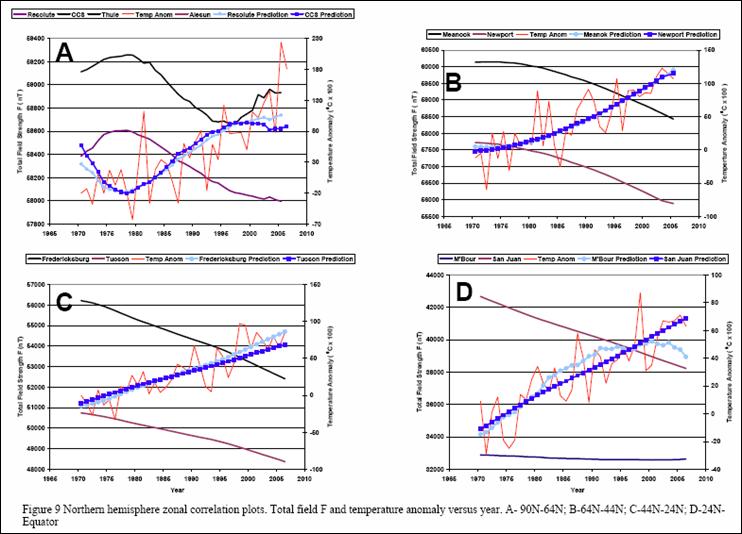
A recent paper (Daniel Johnston: “An Alternative View of Global Warming” May 2008 [http://www.appinsys.com/GlobalWarming/Johnston_MagneticGW.pdf] provides the following figure. He developed a prediction model for predicting the temperature anomaly as a function of the magnetic field. Each frame shows the magnetic field strength at two stations (black and purple) along with the temperature anomaly for the latitude band (red) and the temperature predicted from the magnetic data for the two stations (light blue and dark blue). (Magnetic field strength data comes from http://www.wdc.bgs.ac.uk/)

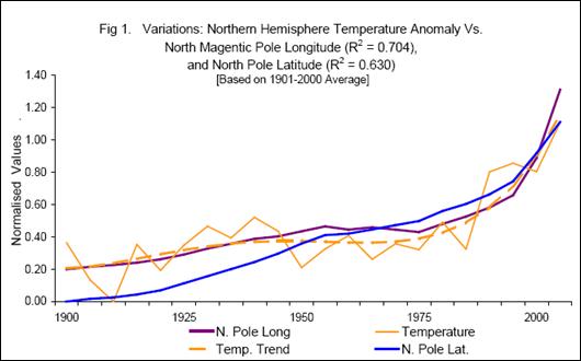
A 2009 paper (Adrian Kerton: “Climate Change and the Earth's Magnetic Poles, A Possible Connection”, Energy & Environment, Vol 20, 2009 [http://www.ingentaconnect.com/content/mscp/ene/2009/00000020/F0020001/art00005] states: “Analysis of the movement of the Earth's magnetic poles over the last 105 years demonstrates strong correlations between the position of the north magnetic, and geomagnetic poles, and both northern hemisphere and global temperatures. Although these correlations are surprising, a statistical analysis shows there is a less than one percent chance they are random, but it is not clear how movements of the poles affect climate.” The following figure is from that paper, comparing normalized NMP location in terms of latitude and longitude with normalized northern hemisphere temperature anomalies.

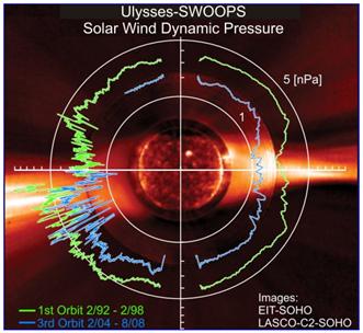
The global cooling over the past several years may be related to the recent decrease in the strength of the solar wind pressure. The following figure (left) shows global measurements of solar wind pressure by the Ulysses satellite (green curves - solar wind in 1992-1998, blue curves - solar winds in 2004-2008). [http://science.nasa.gov/headlines/y2008/23sep_solarwind.htm]  “The average pressure of the solar wind has dropped more than 20% since the mid-1990s … the speed of the million mph solar wind hasn't decreased much—only 3%. The change in pressure comes mainly from reductions in temperature and density. The solar wind is 13% cooler and 20% less dense. The solar wind isn't inflating the heliosphere as much as it used to … That means less shielding against cosmic rays. Ulysses also finds that the sun's underlying magnetic field has weakened by more than 30% since the mid-1990s”

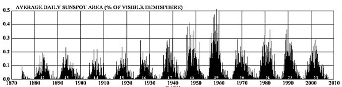
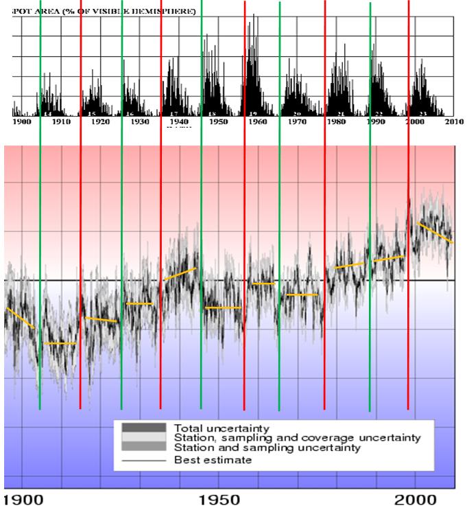
The following figure shows the sunspot cycles since 1880 [http://solarscience.msfc.nasa.gov/SunspotCycle.shtml]. The sunspot cycle is approximately an 11-year cycle – the sun’s magnetic field reverses with each sunspot cycle and thus after two sunspot cycles the magnetic field has completed a reversal cycle – a Hale Cycle – and is back to where it started). Thus a complete magnetic sunspot cycle is approximately 22 years (the 11 year cycle varies substantially). From the solar magnetic flux / sunspot plot shown above it can be seen that the rapid increase in magnetic flux occurs at the onset of the sunspot cycle, a couple of years after the solar minimum occurs.

The following figure compares the Hadley (HadCrut3) global average temperature shown previously with the sunspot cycle since 1900 from above. Shifts in global temperature coincide with the onset of odd-numbered sunspot cycles (red vertical lines). In each case – approximately 1915, 1936, 1957, 1977, 1998 the onset of the odd-numbered cycle corresponds to an increase in global temperature. The onsets of even-numbered solar cycles (green vertical lines) are not as consistent.

A study of solar magnetic clouds during 1994 - 2002 by Wu, Lepping & Gopalswamy, “Solar Cycle Variations of Magnetic Clouds and CMEs” [http://www.scostep.ucar.edu/archives/scostep11_lectures/Pap.pdf] states: “The average occurrence rate is 9 magnetic clouds per year for the overall period (68 events/7.6 years). It is found that some of the frequency of occurrence anomalies were during the early part of Cycle 23: 1. Only 4 magnetic clouds were observed in 1999, and 2. An unusually large number of magnetic clouds (16 events) were observed in 1997 in which the Sun was beginning the rising of Cycle 23”

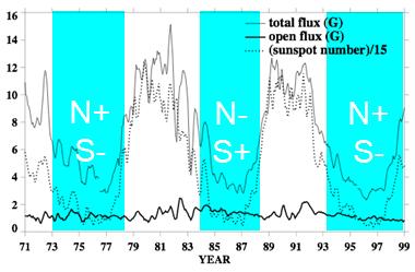
The following figure shows the relative polarity of the Sun’s magnetic poles for recent sunspot cycles along with the solar magnetic flux [www.bu.edu/csp/nas/IHY_MagField.ppt]

A 2007 study (Vovk, V.; Egorova, L., “Role of solar activity in formation of the anomalous El Nin'o current”, Geomagnetism and Aeronomy, Volume 47, Number 1, February 2007 [http://www.ingentaconnect.com/content/maik/11478/2007/00000047/00000001/00001014]) found “a sharp decrease in the SOI indices, which corresponds to the beginning of El Nin'o (ENSO), is preceded one or two months before by a 20% increase in the monthly average Wolf numbers. In warm years of Southern Atmospheric Oscillation a linear relationship is observed between the SOI indices and the number of geoeffective solar flares with correlation coefficients p < −0.5. It is shown that in warm years a change in the general direction of the surface wind to anomalous at the above stations is preceded one or two days before by an increase in the daily average values of IMF Bz. An increase in the SOI indices is preceded one or two months before by a considerable increase in the monthly average values of the magnetic AE indices.”

A 2009 study (Knudsen and Riisager, “Is there a link between the Earth’s magnetic field and low-latitude precipitation?”, Geology, v 37, January 2009 [http://geology.geoscienceworld.org/cgi/content/abstract/37/1/71]) states: “Some studies indicate that the solar modulation of galactic cosmic ray (GCR) particles has profound consequences for Earth's climate system. A corollary of the GCR-climate theory involves a link between Earth's magnetic field and climate, since the geomagnetic field also modulates the GCR flux reaching Earth's atmosphere. In this study, we explore this potential geomagnetic-climate link by comparing a new reconstruction of the Holocene geomagnetic dipole moment with high-resolution speleothem data from China and Oman. The speleothem ¹⁸O data represent proxy records for past precipitation in low-latitude regions, which is a climate parameter that is likely to have been sensitive to variations in the GCR flux modulated by the dipole moment. Intriguingly, we observe a relatively good correlation between the high-resolution speleothem ¹⁸O records and the dipole moment, suggesting that Earth's magnetic field to some degree influenced low-latitude precipitation in the past. In addition to supporting the notion that variations in the geomagnetic field may have influenced Earth's climate in the past, our study also provides some degree of support for the controversial link between GCR particles, cloud formation, and climate.”

A study published in 2008 (Robert Baker, “Exploratory Analysis of Similarities in Solar Cycle Magnetic Phases with Southern Oscillation Index Fluctuations in Eastern Australia” Geophysical Research Papers, Vol. 46, 2008) [http://www3.interscience.wiley.com/journal/121542494/abstract?CRETRY=1&SRETRY=0] states: “There is growing interest in the role that the Sun's magnetic field has on weather and climatic parameters, particularly the ~11 year sunspot (Schwab) cycle, the ~22 yr magnetic field (Hale) cycle and the ~88 yr (Gleissberg) cycle. These cycles and the derivative harmonics are part of the peculiar periodic behaviour of the solar magnetic field. Using data from 1876 to the present, the exploratory analysis suggests that when the Sun's South Pole is positive in the Hale Cycle, the likelihood of strongly positive and negative Southern Oscillation Index (SOI) values increase after certain phases in the cyclic ~22 yr solar magnetic field. The SOI is also shown to track the pairing of sunspot cycles in ~88 yr periods. This coupling of odd cycles, 23–15, 21–13 and 19–11, produces an apparently close charting in positive and negative SOI fluctuations for each grouping. This Gleissberg effect is also apparent for the southern hemisphere rainfall anomaly. Over the last decade, the SOI and rainfall fluctuations have been tracking similar values to that recorded in Cycle 15 (1914–1924). This discovery has important implications for future drought predictions in Australia and in countries in the northern and southern hemispheres which have been shown to be influenced by the sunspot cycle. Further, it provides a benchmark for long-term SOI behaviour.”

The onset of an odd-numbered sunspot cycle (1977-78, 1997-98) results in the relative alignment of the Earth’s and the Sun’s magnetic fields (positive North pole on the Sun) allowing greater penetration of the geomagnetic storms into the Earth’s atmosphere. As mentioned previously “Twenty times more solar particles cross the Earth’s leaky magnetic shield when the sun’s magnetic field is aligned with that of the Earth compared to when the two magnetic fields are oppositely directed” [http://www.nasa.gov/mission_pages/themis/news/themis_leaky_shield.html]